Recently, I went to a local AI hackathon and wrote my first “GPT-wrapper” hackathon idea (a rite of passage!) While doing so, I realised something pretty annoying about the process of working with LLM inference. Writing prompts is not easy! When doing normal programming, if you can’t get something to work, you can look into the documentation, or even dig into the source code. But what do you do when the LLM doesn’t work as you would like? It’s difficult to even determine if

1. The problem is one the model inherently cannot solve
2. You are just prompting wrongly

Even if you do determine that it’s an issue with your prompt, how do you then write a better prompt? As of now, the best resources we have are posts by prompt gurus on the internet, but they generally don’t have much justification for the ideas they present, other than some hand-waving of the technical terms like attention, or “the output had better vibes”.

So this got me thinking. How can we ask the model what the best prompt should be? The first-instinct answer would be to say: “Oh, just ask the model!” However, that assumes the model has a good understanding of its inner workings, or has some ability to “introspect”. Neither of which should be trained into the model through next-token prediction from internet text.

Instead, we could think about another method to “ask” the model, backpropagation!

General idea

Generally, when we want to use LLMs to solve specific problems, beyond prompting, the next option is usually fine-tuning. With fine-tuning, we gather a dataset that represents our task, and train the model to better fit our custom dataset. This is usually done by calculating the loss of the outputs generated by the model, and backpropagating the loss to find the gradient of the weights of the model.

               /---<-- gradient <---+
          +---------+               |
Inputs -> | Weights | -> Output -> Loss
          +---------+
              LLM

We then use these gradients to tweak the weights of the model such that our loss slowly decreases, thus improving model performance on the task.

What if we don’t want to change the weights of the model? What happens if we backpropagate to the input instead?

   +--------<----- gradient ----<---+
   |      +---------+               |
Inputs -> | Weights | -> Output -> Loss
          +---------+
              LLM

For some tasks, our input can actually be conceptually broken down into two portions, the prompt and the “true” input. For example, consider the task of code generation, our inputs could look like so:

       [            Prompt                ] ["True" Input]
Input: Please generate some Python code for the game pong
Output: def pong(): ...

       [     Prompt       ] ["True" Input]
Input: In python, implement the game pong
Output: def pong(): ...

So if we knew the gradient of our input as a whole, we could also determine the gradient of the prompt portion alone. If we tweak this, just like how we would with the model weights, could we generate an optimal prompt for our specific task?

Let’s test it out

To test this out, we need to make a few decisions.

1. What downstream/specific task are we trying to optimise for?
2. What model do we use?

Task selection

As a proof-of-concept, I wanted to think of a simple language task that the model should be capable of solving. By restricting to language tasks, we can be more confident that any issues would be due to the prompt rather than the model itself being incapable of solving the task. This is in comparison to more complicated tasks like reasoning, where we aren’t even sure if the model is capable of solving them with an optimal prompt.

The task I decided on was determining the antonym of words. The antonym of a word is essentially just another word that has an “opposite” meaning of the word. For example, the antonym of “good” is “bad”. Symmetrically, the antonym of “bad” is “good”. Not only is this a rather simple language task, it’s also a task where there are public datasets.

To use an LLM to solve this problem, we can phrase a prompt like so:

Here are two antonyms <word1> and <word2>

We feed in only the prefix Here are two antonyms <word1> and into the model, and make the model infer its guess of <word2>. To frame it as a prompt optimisation problem, we can then blank out of the word antonym!

Here are two <blank> <word1> and <word2>

We initialise <blank> to some random token embeddings, and try to finetune with many antonym pairs from our dataset. As training loss decreases (hopefully 🤞), our <blank> should contain more semantic meaning that describes the task we want to solve. More interestingly, we can also see if we actually end up with the word “antonym” in the end!

Model selection

But what about model selection? We don’t even need to consider closed-source models since we are using this weird finetuning process. But even among the open-source models, we are spoiled for choice. My intuition for this was to select the smallest (by parameter size) transformer-era model that could provide some meaningful results for the antonym task.

Playing around with a few models on huggingface, I found that GPT-2 Large seemed to fit the bill. GPT-2 Large only has 774M parameters (very small by todays standards) and seemed to perform okay when provided the input Here are two antonyms <word1> and. The smaller model I considered, GPT-2, did not seem to provide good inference for this task.

With these two things decided, we can get to work on training!

Training Arc

First, we had to wrap the existing GPT-2 model to introduce our tunable prompt (the <blank> described above).

class GPT2PromptModel(torch.nn.Module):
    gpt2: GPT2LMHeadModel
    prompt: torch.Tensor
    prompt_len: int

    def __init__(self, prompt_len: int, gpt2):
        super(GPT2PromptModel, self).__init__()
        self.gpt2 = gpt2
        # freeze gpt2 parameters
        for parameter in self.gpt2.parameters():
            parameter.requires_grad = False
        # tunable prompt
        embed_dim = self.gpt2.transformer.embed_dim
        embed_weight = self.gpt2.get_input_embeddings().weight
        self.prompt = torch.nn.Parameter(torch.normal(
            embed_weight.mean(axis=0).broadcast_to(prompt_len, embed_dim),
            embed_weight.std(axis=0).broadcast_to(prompt_len, embed_dim)
        ))
        self.prompt_len = prompt_len

    def forward(
        self,
        prompt_index: int,
        input_ids: Optional[torch.LongTensor] = None,
        inputs_embeds: Optional[torch.FloatTensor] = None,
        **kwargs
    ):
        if input_ids is not None and inputs_embeds is not None:
            raise ValueError("You cannot specify both input_ids and inputs_embeds at the same time")
        elif input_ids is not None:
            wte = self.gpt2.get_input_embeddings()
            inputs_embeds = wte(input_ids)
        elif inputs_embeds is None:
            raise ValueError("You have to specify either input_ids or inputs_embeds")
        # Insert tunable prompt
        batch_sz = inputs_embeds.shape[0]
        inputs_embeds[:,prompt_index:prompt_index + self.prompt_len,:] = self.prompt.broadcast_to((batch_sz,) + self.prompt.shape)
        return self.gpt2(inputs_embeds=inputs_embeds, **kwargs)

There were two interesting details for this wrapper implementation, prompt initialisation and the modified forward pass.

In order to store a trainable prompt, it must be stored in a form that can be backpropagated to. That means that we can’t just store a string like ' antonym' and hope that the model changes it. To understand this, we we can look at the intial phase of how we feed strings into a model.

String:       "Lord_Idiot"
Tokens:       [ "Lord", "_", "Id", "iot"]
Token ids:    [ 22438,  62,  7390, 5151 ]
Token embed.: [
                [0.12, -0.1, ...],
                [0.01,  0.3, ...],
                [0.20,  0.7, ...],
                [0.11, -0.1, ...]
              ]

Since none of these steps are differentiable, we can only backpropagate till the token embeddings. This means that our trainable prompt should be stored in its embedding form. Knowing the form, then what about the initial value of the prompt? This is important as poor parameter initialisation could affect training outcomes.

There’s lots of literature about initialisation of weights, but what about initialisation of … prompts? While there isn’t much material about that, we can use some intuition to guide the process.

During the pre-training for the GPT-2 model, its inputs were always embeddings from the vocabulary of the tokenizer. Therefore, the weights of the model should be trained to perform well for this vocabulary. Consequently, we would want our prompt embeddings to be similar to the vocabulary, i.e. in-distribution with respect to the embedding table. We also want some level of randomness so that we don’t have a static starting point for every training run. To achieve this, we can use the embedding table mean and standard deviation for each embedding dimension (across the 50257 tokens in the vocabulary) as the parameters for a normal distribution. With that, we can generate random token embeddings that are in-distribution with respect to the vocabulary.

For the forward pass of the model, we add an additional argument prompt_index that describes where the tunable prompt should be inserted into the text provided to the forward pass. This essentially describes where in the text we replace with our <blank>. Then, we make sure to run the input through the embedding layer first, and substitute our tunable token embeddings at the correct indices. The resulting embeddings are then passed into the GPT-2 model as usual.

Results

Before seeing the training results, it would be good to see the test loss for the original prompt.

Prompt:          "Here are two antonyms <word1> and"
Expected output: " <word2>"

We test this static prompt on our test data.

class Wrapper(torch.nn.Module):
    gpt2: GPT2LMHeadModel
    
    def __init__(self, gpt2):
        super().__init__()
        self.gpt2 = gpt2

    def forward(self, _, **kwargs):
        return self.gpt2(**kwargs)

test_model(Wrapper(gpt), test_loader, gpt_tokenizer)
# 4.4749 (test loss)

Now, we train a new prompt to replace antonyms on the training set, and watch as loss converges :D

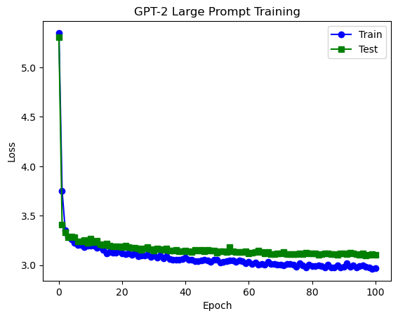
We can see that we actually went overkill on training. Within about ~10 epochs on the training set (about ~5000 pairs of antonyms), we already reach a plateau for our test loss. When we compare this to the original prompt, we actually achieve far better performance with a loss of around ~3.1. This was very impressive to me, and I wanted to see how well the model actually performed, so I tried a few generations using the model.

Actual: Here are two antonyms scatter and crowd
Predicted: Here are two <prompt> scatter and gather

Actual: Here are two antonyms flat and uneven
Predicted: Here are two <prompt> flat and curved

Actual: Here are two antonyms unpack and pack
Predicted: Here are two <prompt> unpack and pack

Actual: Here are two antonyms extinct and active
Predicted: Here are two <prompt> extinct and extant

Actual: Here are two antonyms mind and forget
Predicted: Here are two <prompt> mind and body

Actual: Here are two antonyms disarm and arm
Predicted: Here are two <prompt> disarm and disarm

The results seemed really amazing! We see that the model really does display traits of generalising to the task. Notice that even when it disagrees with the test set (e.g. “flat” and “uneven”), its wrong answer “curved” is actually a valid antonym for flat! Similarly for extinct and extant.

However, there are some times where the model seems to parrot <word1>, like you can see for the last example “disarm”. This is something that I noticed in a decent percentage of the generated outputs. Nevertheless, I’d consider this a successfully trained prompt.

Interpretability?

Earlier, I alluded to the idea that we could subsequently try to identify if the prompt that we train actually maps back to a real word/sentence. By using cosine similarity with the embedding table, I tried to match the trained prompt with the closest vocabulary tokens.

token_id: 39686, token: "sounding", cosine similarity: 0.22011171281337738
token_id: 30439, token: " unintention", cosine similarity: 0.21060492098331451
token_id: 9364, token: "ÃÂÃÂÃÂÃÂ", cosine similarity: 0.19043108820915222
token_id: 14606, token: " aest", cosine similarity: 0.147452250123024

Unfortunately, it didn’t seem to be very useful. There’s not much meaning to the sentence:

Here are two sounding unintention ÃÂÃÂÃÂÃÂ aest <word1> and <word2>

However, this result seems unsurprising when you look at the cosine similarity of the tokens. Every token has a very low cosine similarity to even its closest vocabulary token (closest would be similarity 1), so it seems that the prompt we generated does not fit well in the vocabulary, thus generating nonsense.

Optimization?

Before moving on to more experiments, I wanted to address one big issue - performance. Training on GPT-2 seemed to run really slow! This makes sense considering we are running similar computations as a fine-tuning/training run of the whole model. Nevertheless, we do want faster computations if we want to experiment more.

I’d learnt recently about FlashAttention, which is a custom algorithm + accompanying fused CUDA kernels which makes some tradeoffs for better real-world performance of the transformer attention block. Flash attention wasn’t supported for GPT-2 on huggingface at the point I did this, but a candidate implementation was on the dev branch so I tried it out. Unfortunately, it didn’t seem to improve performance much.

Instead, what actually improved performance was mixed precision training. Our model is usually loaded with “full”-precision float32 parameters. Every operation is thus done between 32-bit floating points. If we change the parameters to float16 instead, we could use faster operations on the GPU instead!

However, using float16 didn’t work in my case as I was facing a lot of numerical overflow issues (since float16 has a reduced range of numbers it is able to represent). What did work was bfloat16, which is another 16-bit floating point representation which has almost equal range to float32, but lower fractional precision than float16. This greater range prevented the numerical overflow issues, while giving me a big boost in performance (from 2minute epochs to ~30seconds, about 4x speedup).

Better Interpretability

Now that we can train faster, I wanted to revisit the idea of interpretability. Earlier, we represented each trainable prompt token as a 1280-dimension embedding. Then after training, we try to map this embedding to the closest one in the embedding table. This didn’t work well because there are no guardrails to ensure that the trained embedding would map to one of the vocabulary tokens. This begs the question, is there a way to guarantee this?

Let’s revisit the idea of tokenisation again. Earlier, this was how I described the tokenisation process:

String:       "Lord_Idiot"
Tokens:       [ "Lord", "_", "Id", "iot"]
Token ids:    [ 22438,  62,  7390, 5151 ]
Token embed.: [
                [0.12, -0.1, ...],
                [0.01,  0.3, ...],
                [0.20,  0.7, ...],
                [0.11, -0.1, ...]
              ]

However, we could actually add an additional step better represent the tokenisation process:

Token:         "_"
Token id:      62
Token one-hot: [0, 0, 0, ..., 1, ... 0, 0, 0]
Token embed:   [0.01, 0.3, ...]

Going from a token id to its one-hot representation is just creating an tensor of 0s, and replacing the ith element with 1. Then this one-hot representation could be matrix multiplied with the embedding matrix to get the actual token embedding. This gave me an idea: Could we force our parameter to be one-hot, while still being differentiable?

Perhaps we could represent our token as a 50257-dimension tensor and then run it through a softmax! The softmax wouldn’t ensure that it is one-hot, but would ensure that the elements sum to 1, which is closer to an approximation of a one-hot vector. If we exaggerate the differences between the elements in the vector, hopefully we can force the resulting softmax to have a single high-value index.

Unfortunately, this method of training didn’t seem to converge, and rather got stuck on its initialised values. It seems interpretability of our prompt will remain a mystery for now.

Sample efficiency

During training, we use about 5000~ antonym pairs, but is this really necessary? Perhaps we would be able to determine a prompt from lesser examples (recall that earlier, the concept of antonyms was only explained with two examples).

To test this, I tried to train with 100 training examples instead. Amazingly, we can train a pretty good prompt that generalises, even with only 100 training samples:

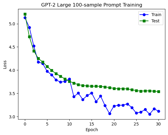
To get a sensing for the performance, here are some example outputs:

Actual: Here are two antonyms knockout and decision
Predicted: Here are two <prompt> knockout and knockout

Actual: Here are two antonyms heterogeneity and homogeneity
Predicted: Here are two <prompt> heterogeneity and uniformity

Actual: Here are two antonyms widening and narrowing
Predicted: Here are two <prompt> widening and narrowing

Actual: Here are two antonyms incapable and capable
Predicted: Here are two <prompt> incapable and capable

Actual: Here are two antonyms refreshing and old
Predicted: Here are two <prompt> refreshing and depressing

Actual: Here are two antonyms shy and bold
Predicted: Here are two <prompt> shy and bold

Actual: Here are two antonyms plain and decorated
Predicted: Here are two <prompt> plain and complex

Pretty cool!

Final thoughts

Overall, I think this was a pretty successful experiment! I don’t know if this would be a particularly practical technique, considering that the computation necessary is similar to that of finetuning. Nevertheless, I’m happy to see that it kind of works, and I’m curious to see if it can work for more complicated tasks as well.

Edit: Seems this concept is called prefix-tuning! A much more in-depth paper about this here.

If you’re interested to check out the code for this project, I’ve uploaded it on my github.